Bayes Rule - An Example with Code
In the interests of learning and developing a better sense on how to to use Bayes Rule we’re going to do two things in this post.
- We’re going use Bayes Rules to come up with an analytical solution to a probability problem (like you’d see in an interview setting).
And
- We’ll simulate some data to see if we can approximate an analytical solution (to help develop our programming chops).
The Scenario
Imagine you’re a patient who has just received a positive test result for HIV. Horrified, you know false positives are possible so you set out to calculate what is the probability of having HIV given you tested positive i.e. what is $\color{black}P(HIV|+)$?
Available to you are a couple more pieces of information:
-
The prevalence of HIV in the population:
- $\color{black}P(HIV) = 0.0001$ (.01%)
-
The probability of testing positive given you have HIV:
- $\color{black}P(+|HIV) = 0.999$ (99.9%)
Leveraging Bayes Rule
If you haven’t heard of Bayes Rule it’s essentially a way to reason about conditional probabilities.I think the easiest way to remember it is to just use some mathematical symmetry. If you recall the formula for the joint probability of two dependent variables we get the following:
$$ \color{black}P(HIV \cap +) = P(HIV|+)*P(+) $$
The neat (and symmetric) thing about that joint probability is we can also write the it like this:
$$ \color{black}P(+ \cap HIV) = P(+|HIV)*P(HIV) $$
And with some substitution $$ \color{black}P(HIV|+)*P(+) = P(+|HIV)*P(HIV) $$ then rearrangement and we now have a formula for calculating our conditional probability through Bayes Rule! $$ \color{black}P(HIV|+) = \frac{P(+|HIV)*P(HIV)}{P(+)} \tag{1} $$
I can introduce some terms here about priors, posteriors, and likelihoods but I’ll refrain in the interests of brevity; just know that these terms are related to quantities in equation (1).
The Analytical Solution
Combining the data supplied to us in the scenario with equation (1) and the only real thinking we have to do is derive our denominator $\color{black}P(+)$ from Bayes Rule and we’ll be able to generate our probability of interests.
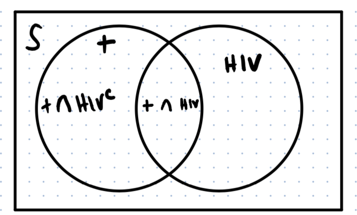
To derive $\color{black}P(+)$ you have to think about the Law of Total Probability. The law states that you can find a probability by summing up the intersections of it’s disjoint sets and here’s a Venn Diagram for a visual:

As you can see from the visual above (and invoking the Law of Total Probability), our probability of interests can be defined as:
$$ \color{black}P(+) = P(+ \cap HIV) + P(+ \cap HIV^\mathsf{c}) $$
We can break down this equation down a bit further
$$ \color{black}P(+) = P(+|HIV)*P(HIV) + P(+|HIV^\mathsf{c})*P(HIV^\mathsf{c}) $$
And with one last rearrangement to make it very apparent how to derive this quantity and we’re left with this:
$$ \color{black}P(+) = P(+|HIV)P(HIV) + (1-P(+|HIV))(1-P(HIV)) $$
All we have to do now is plug and chug to generate our probability of interests, $\color{black}P(HIV|+)$. And here’s the solution if you haven’t tried yourself yet:
$$ \color{black}P(HIV|+) = \frac{P(+|HIV)P(HIV)}{P(+|HIV)P(HIV) + (1-P(+|HIV))(1-P(HIV))} $$
Now, substituting in our know quantities and we get:
$$ \color{black}P(HIV|+) = \frac{0.9990.0001}{0.9990.0001 + (1-0.999)(1-0.0001)} $$
Which evaluates to $\color{black}P(HIV|+) = 0.09083$. And there we have it, the analytical solution to our problem using Bayes Rules. Now lets see if we can approximate this solution with some simulated data.
The Code
There’s a few things to note about this simulation.
-
This is a two stage data generation process. First you simulate data for people with HIV then you simulate whether those people will test positively.
-
We’re going to need to generate a large number of samples because of the low prevalence of HIV in the population (0.01%).
And
- Because doing one simulation of the data generation process would just give us a single point estimate (i.e. the mean), we’re going to do multiple simulations to generate a distribution of means then take the mean of that distribution as our approximation of the probability (think of the central limit theorem).
So, rather than expanding too much on the code, I’ll leave it here with some comments.
from joblib import Parallel, delayed
from numpy.random import binomial as rbinom
from numpy import array, empty, isclose

# Our given data
p_positive_g_hiv = 0.999
p_hiv = 0.0001
p_not_hiv = 1 - p_hiv
p_positive_g_not_hiv = 1-p_positive_g_hiv

# Patient population sample size
hiv_ss = 2e6 # 2 million

# How many 'simulations' to run
distr_ss = 400

def sample(pop_ss=hiv_ss):
    """
    Function to simulate and estimate a single mean for the P(HIV|+).

    :param pop_ss: Sample size of the population we're simulating
    i.e. how many people are we testing for HIV & testing
    :type pop_ss: int
    """
    hiv = rbinom(1, p_hiv, int(pop_ss))
    test = empty(int(pop_ss))
    test[hiv==0] = rbinom(1, p_positive_g_not_hiv, test[hiv==0].shape)
    test[hiv==1] = rbinom(1, p_positive_g_hiv, test[hiv==1].shape)
    return hiv[test==1].mean()


def run_parallel(func, n_runs, n_jobs=4):
    """
    Wrapper for parallel processing a function
    (with default args/kwargs).

    :param func: Function to parallel process
    :type func: func
    :param n_runs: Number of times to execute function
    :type n_runs: int
    :param n_jobs: Number of cores to use
    :type n_jobs: int
    """
    return array(
        Parallel(n_jobs=n_jobs)(delayed(func)()
        for _ in range(distr_ss))
    )


# Took about 24s on my 2015 macbook air
distr = run_parallel(func=sample, n_runs=distr_ss)

# Check our approximation to the real answer
p_test_postive = p_positive_g_hiv*p_hiv + p_positive_g_not_hiv*p_not_hiv
p_hiv_g_positive = (p_positive_g_hiv*p_hiv)/p_test_postive

assert isclose(
       distr.mean(),
       p_hiv_g_positive, atol=0.001
), "Not a good approximation"
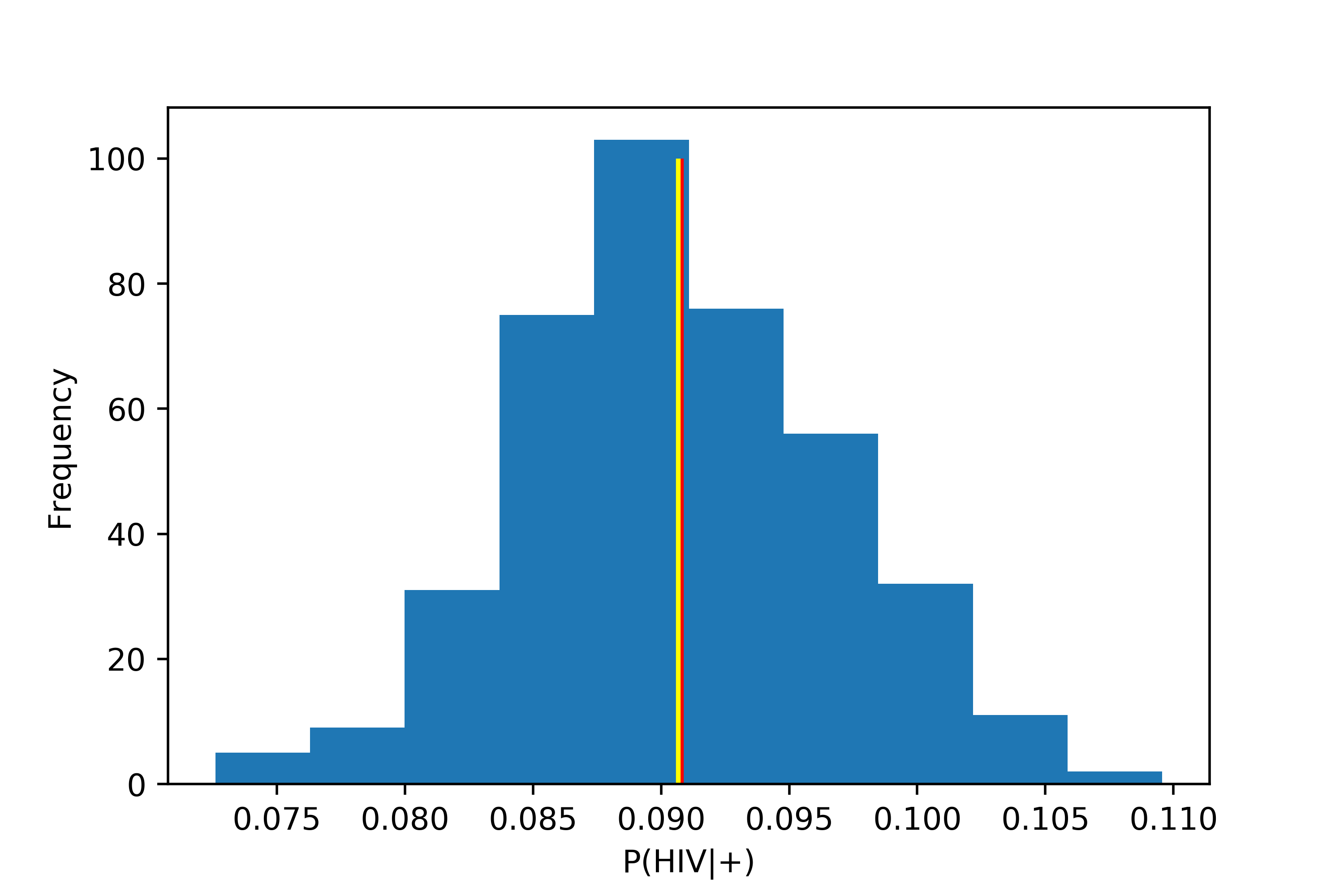
So there we have it. In the image below I’ve visualized the distrubtion of means we created from the code above. The true probability is marked by a vertical line in red and our approximation is marked with yellow vertical line.

Feel free to comment, play with the code, and make some more interesting plots. Thanks for reading and I hope you enjoyed.