Feature Engineering for Maching Learning - Post 1 of 7
- This is Part 1 of 7 in my series on the book,‘Feature Engineering for Machine Learning’ *
It’s been a little while since I added some content to my blog but it isn’t for lack of learning. After reflecting on what I’ve done to get where I am now, I decided it’s time to go back through backlog of notes, links, and documents and turn them into proper blog posts. For full disclosure, I did leverage AI in these series of posts to follow, however, all sketches, perspectives, and thoughts are novel; I simply asked my SolveIt instance to help me take my 91 page google doc of notes and images and turn them into structured posts.
That said, the tone of the posts are in line with my writing and all content has been reviewed & edited by me. Lastly, these post would not have been possible were it not for the book club I led while working at Doximity; thanks to all those who contributed:
- Tai Nguyen
- Victor Kofia
- Kevin Studer
- Nana Wu
- Joseph Lin
- Chip Hollingsworth
- And others I may have forgot to mention
Enjoy the following series and for context, we read this book at the tail end of 2020, so while the content may not be as hot as LLM’s, it’s great foundational material for machine learning.
Taming Numbers: Counts, Scaling, and When They Matter
After working through the first couple chapters of Feature Engineering for Machine Learning, I really wanted to centralize all the subtlties related to how we represent and transform our data before any of it ever sees a model. This post covers some of these foundations: how to deal with counts, when and why to scale your features, and some of the gotchas that nobody warns you about until you’ve already shipped something questionable.
Setting the Stage: Scalars, Vectors, and Spaces
Before diving into transforms, it’s worth grounding ourselves in the language we’ll be using. Features live in vector spaces, and the way we manipulate those spaces matters.
In the example below, we’re viewing the row and column spaces of our data & features as well as how to represent them geometrically. Something that isn’t represented is the NULL space and that can be considered a space where vectors can’t reach.
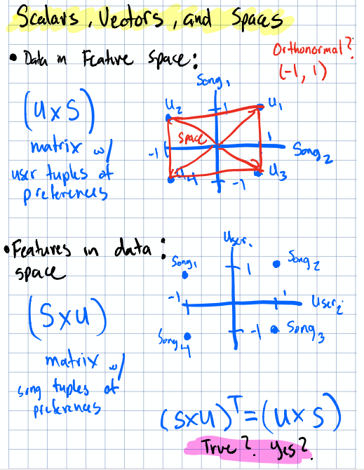 Overview of scalars, vectors, and the spaces they inhabit.
One thing that tripped me up early on was the relationship between transposing a matrix and taking its inverse. They’re not the same thing and you can think of the transpose as flipping a matrix along the diagnol, there is no stretching of vectors occuring, and an inverse as undo-ing a transformation (e.g. unflipping & unstretching). For orthogonal matrices (where all vectors are perpendicular) & orthonormal matrices (where rows and columns are all unit-length and perpendicular to each other), the transpose does equal the inverse. That’s a special property, and it comes up more than you’d think in dimensionality reduction and decompositions. Worth filing away.
Dealing with Counts
Binarization: Sometimes Less Is More
Here’s a scenario I’ve actually dealt with: you’re looking at video play counts for users on a content platform. Sounds straightforward, right? But what if some users have autoplay enabled and a video is just looping on their screen while they’ve walked away to make coffee? Suddenly your “engagement” metric is wildly inflated for certain users.
 The binarization transform — collapsing counts to binary signals.
Binarization is converting counts to simple 0/1 indicators, is one way to add robustness against this kind of engagment inflating noise. Instead of asking “how many times did this user play a video?” you ask “did this user play a video at all?” It’s a blunt instrument, sure, but sometimes blunt is exactly what you need.
The tricky part is knowing when binarization is the right call versus some other transformation. It’s more of a gut check and domain intuition than a rigorous statistical test. You could, for instance, compare users without autoplay enabled against a binarized version of everyone’s counts and see if your downstream metrics align. But the book doesn’t really hand you a formal test for this, it’s more about shaping your intuition, which I think is actually the right lesson.
Large Magnitudes: When Your Features Fight Each Other
This section I found interesting from a practical standpoint. Imagine you’re fitting a linear model and one feature ranges from 0 to 10 while another ranges from 0 to 1,000,000. Can those large magnitudes actually affect the stability of your coefficient estimates?
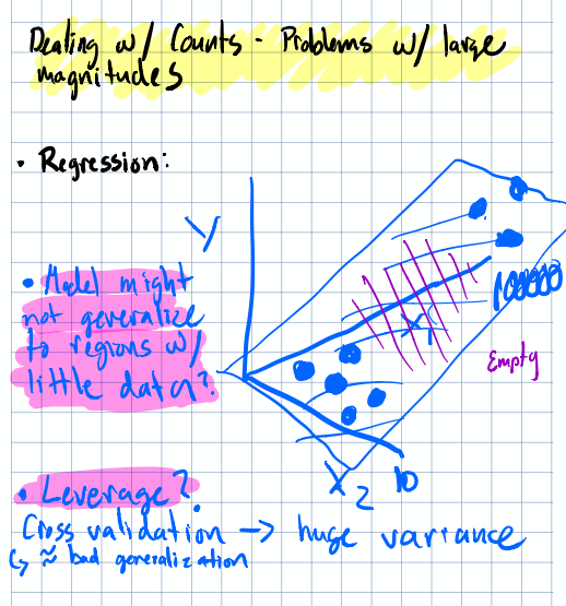 Visualizing the problem of large magnitudes in feature space.
The short answer is yes. Large magnitudes can create numerical instability, especially in algorithms that rely on gradient descent or distance calculations. The empty regions of your feature space become vast, and the algorithm struggles to navigate efficiently.
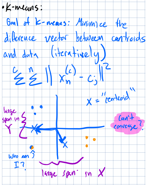 How large magnitudes can affect convergence.
Now here’s the interesting bit: not all algorithms care equally. Random forests partition the feature space with splits, so they’re largely immune to magnitude issues. But if you’re working with an existing model and trying to introduce new features with very different scales, you absolutely need to think about this. Will the new features throw off the balance your model already found?
This is the kind of thing worth simulating; take your existing feature set, toss in or scale a feature with wildly different magnitude, and see if convergence degrades. It’s a small experiment that could save you a lot of headaches.
Quantization and Binning: The Art of Discretization
Binning is where things get philosophically interesting. You’re taking continuous data and chopping it into buckets but how you chop matters a lot.
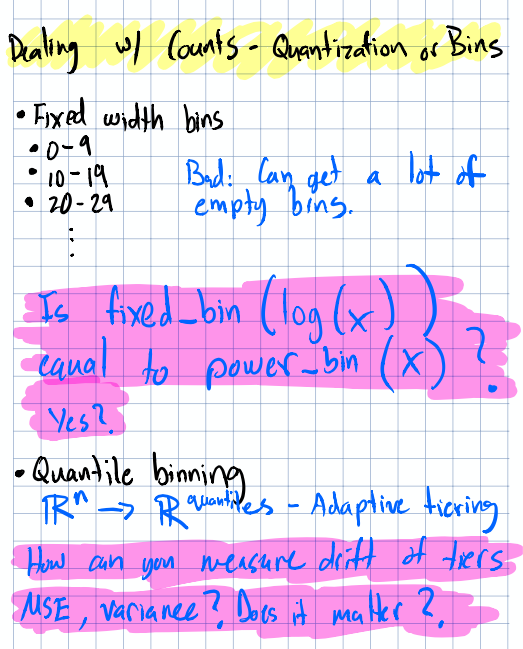 Different approaches to binning continuous features.
Take a concrete example: you want to tier users by how many digest emails they read per week. You could do fixed-width bins (0–5, 5–10, 10–15, …) or quantile-based bins that evenly split your distribution. Quantile binning is arguably more “robust” because it gives equal weight to all parts of the distribution — but does that always lead to better insights than ad-hoc binning based on human understanding?
Think about it: if you know that reading 1–2 emails versus 3+ emails represents a meaningful behavioral difference, a quantile split might blur that boundary. Sometimes domain knowledge should override statistical elegance.
One question that stuck with me: is fixed_width_binning(log(x)) with a bin width of 1 the same as power_binning(x) in base 10? It’s a fun exercise to prove (or disprove) with a bit of code — and the answer tells you something about the relationship between logarithmic and exponential scales.
Log Transforms: Making the Ugly Beautiful
Log transforms are the workhorse of feature engineering, and for good reason. When you have right-skewed count data (which is… most count data), taking the log can pull things into a much more well-behaved distribution.
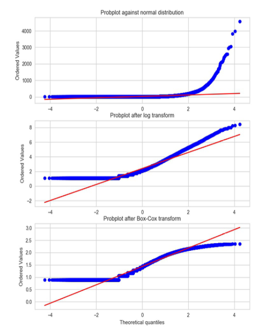
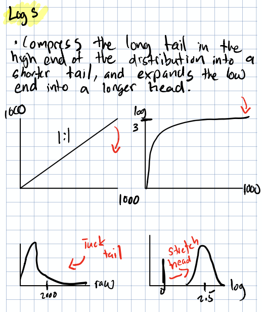 Q-Q plot showing how log transforms improve normality. The bottom panel shows the optimal $\lambda$ for the Box-Cox transform, chosen by maximizing the MLE of the parameter.
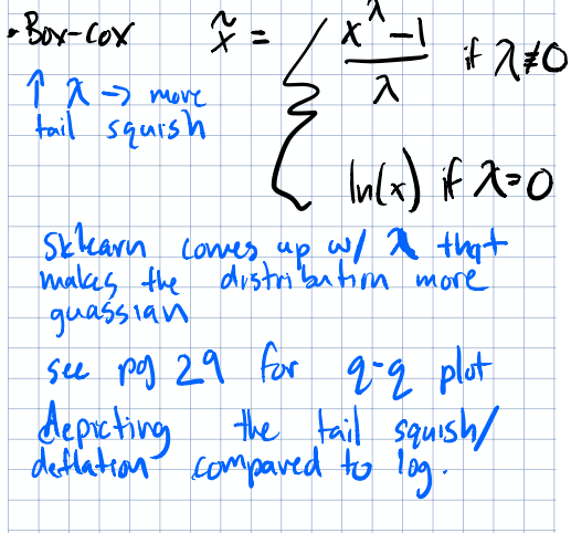
The Box-Cox transform generalizes this idea. Instead of just taking $\log(x)$, you apply:
$$\tilde{x} = \begin{cases} \frac{x^\lambda - 1}{\lambda} & \text{if } \lambda \neq 0 \ \ln(x) & \text{if } \lambda = 0 \end{cases}$$
The optimal $\lambda$ is chosen to make the transformed data as close to normal as possible. When $\lambda = 0$, you recover the plain log transform. It’s neat but it also raised a question about what’s the statistical test to rigorously measure whether the log transform or the Box-Cox actually made your data “more normal”? It’s worth looking into if you’re curious.
Feature Scaling
Now we get to the heart of the chapter. You’ve cleaned up your counts, maybe logged them — but your features are still on wildly different scales. Here’s the toolkit.
Min-Max Scaling
The simplest approach: squash everything to $[0, 1]$:
$$\tilde{x} = \frac{x - min(x)}{max(x) - min(x)}$$
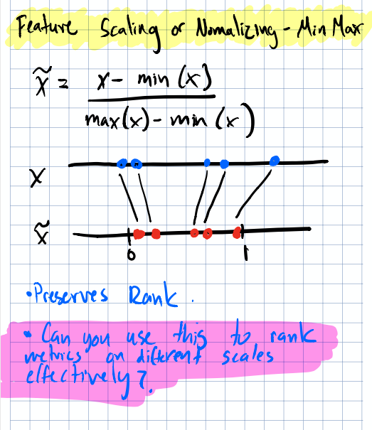 Min-Max scaling maps features to the $[0, 1]$ range.
I’ve seen a clever variation of this in ad ranking systems. When you have bids for engagements on similar scales but you need to differentiate them because maybe each ad wave represents a higher paid product, you can add a constant to one set of bids to create clean tiers:
- $X + 100$ puts $X$ on the range $[100, 101]$
- $Y$ stays on $[0, 1]$
This guarantees that $X$-type bids always rank above $Y$-type bids, which may be the business logic you need.
But the question remains: what are the cons of putting different scales on a 0–1 span? Are there numerical edge cases or unforeseen scenarios where this breaks down? Worth thinking about, especially with outliers that can compress the bulk of your data into a tiny portion of the range.
Standardization (Z-Scores)
Center your distribution around zero and scale by standard deviation:
$$\tilde{x} = \frac{x - \bar{x}}{\hat{\sigma}_{x}}$$
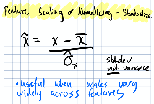 Standardization centers the distribution at zero with unit variance.
This is the go-to when you want to put different entities on the same scale for comparison. It preserves the shape of your distribution (unlike min-max, which can be distorted by outliers) and is what most people mean when they say “normalize your features” in casual conversation.
L2 Normalization
Project each sample onto the unit circle (or hypersphere):
$$\tilde{x} = \frac{x}{||x||^2}$$
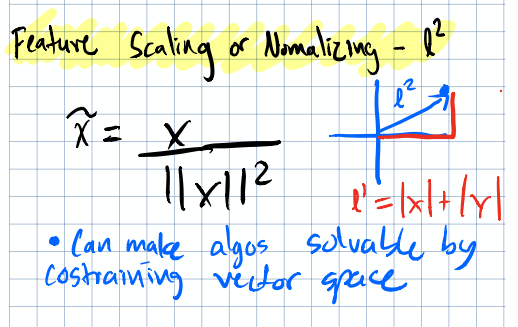 L2 normalization projects data onto the unit circle.
This is especially useful when the direction (vector orientation) of your feature vector matters more than its magnitude (vector size), think text data, where document length shouldn’t dominate the signal… a document’s topic should similar regardless of 10,000 words of 100 words; the words themselves are what matter.
Feature Selection: A Brief Note
The chapter wraps up with a nod toward feature selection and reducing the number of features to improve model performance and efficiency.
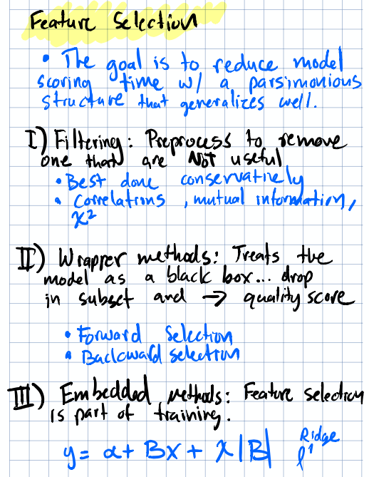 Summary of feature selection considerations.
One thing that bugged me… the book emphasizes reducing model scoring time rather than training time. At first that seems backwards because training is the expensive part, right? But in production, you score way more often than you train. A model that’s slightly slower to train but faster to score can save significant compute at scale. It’s a production mindset, and I wish the book had expanded more on feature selection techniques beyond this brief mention.
Takeaways
The biggest lesson from these first two chapters isn’t any single technique, it’s that feature transformations don’t add new information. Scaling, binning, logging; none of these create signal that wasn’t there before. What they can do is:
- Remove noise that obscures the signal (binarization, log transforms)
- Improve numerical stability so your algorithm can actually converge (scaling)
- Speed up computation by putting features on comparable scales (normalizing)
- Match the assumptions of your chosen algorithm (normality, bounded ranges)
The art is in knowing which transformation serves your specific problem and that requires understanding both the math and the domain. No single recipe works every time.
Next up in Part 2: we’ll dive into the world of text features; bag-of-words, n-grams, and the surprisingly deep rabbit hole of turning language into numbers.