Feature Engineering for Maching Learning - Post 2 of 7
- This is Part 2 of 7 in my series on the book, ‘Feature Engineering for Machine Learning’ *
Text as Features: From Bag-of-Words to Phrase Detection
When I first dug into this chapter on text featurization, I kind of wished the author had put the summary at the beginning. I found myself guessing about applicable workflows for a good chunk of the reading; when would I reach for bag-of-words vs. n-grams vs. something fancier? It wasn’t until the end that the full picture clicked. So let me try to save you that suspense and lay things out a bit more intuitively here.
The core idea of this chapter is deceptively simple: how do you turn messy, hierarchical, human text into numbers a model can use? The answer, it turns out, involves a spectrum of techniques that trade off simplicity for richness.
The Big Tradeoff
The first thing to internalize is text is highly structured and when you turn structured text into a vector of word counts, you lose all of that; hierarchy, parts of speech, dependencies between words are all gone, just like that. What you’re left with is a big ole vector of counts or relative frequencies, depedening on what you’re doing.
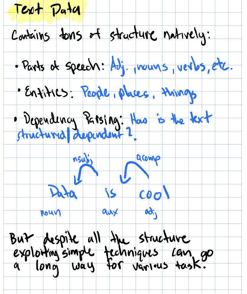 Overview diagram for text features from the chapter intro
The more I thought about, the more I wondered, is losing all that structure a bad thing? Not necessarily. It depends entirely on your task. But it’s important to understand what you’re giving up when you featurize text, because that awareness shapes every decision downstream.
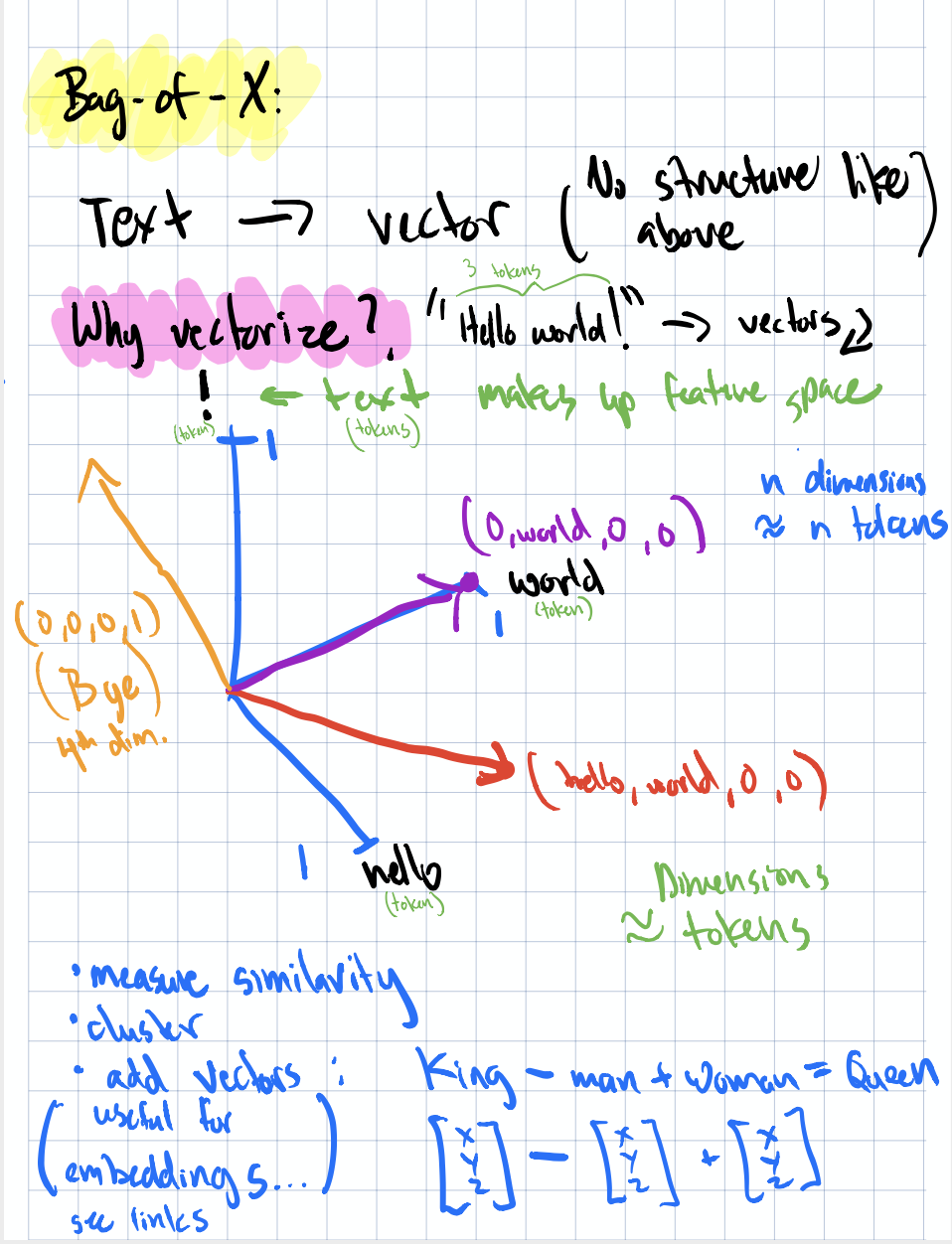 Text to vectors and their utilities
And while a lot of the methods presented in this chapter transform away some, if not all, structure, know there exists other transformations that can maintain higher levels of structure such as semantics. The famous “king - man + woman = queen” magic embodies that text representation where similarity of vectors can surface much more relevant information but deriving that perspecitve is much more computationally complex than basic counts and frequencies. So is it worth it? It all depends on what you’re trying to do.
In the rest of the post we’ll go over the various methods for featurizing text, starting with the simplest and getting progressively more complex. And we’ll round it out with a summary of how to combat one of the main issues with text featurization; sparsity, the larger your data, the sparser your feature space… unless you implement some mitigation techniques as we’ll describe later on.
Bag-of-Words
Bag-of-words (BOW) is the simplest approach: tokenize your text, count up each word, and you’ve got a feature vector. Each unique word in your vocabulary becomes a dimension, and the value is how many times that word appeared in the document.
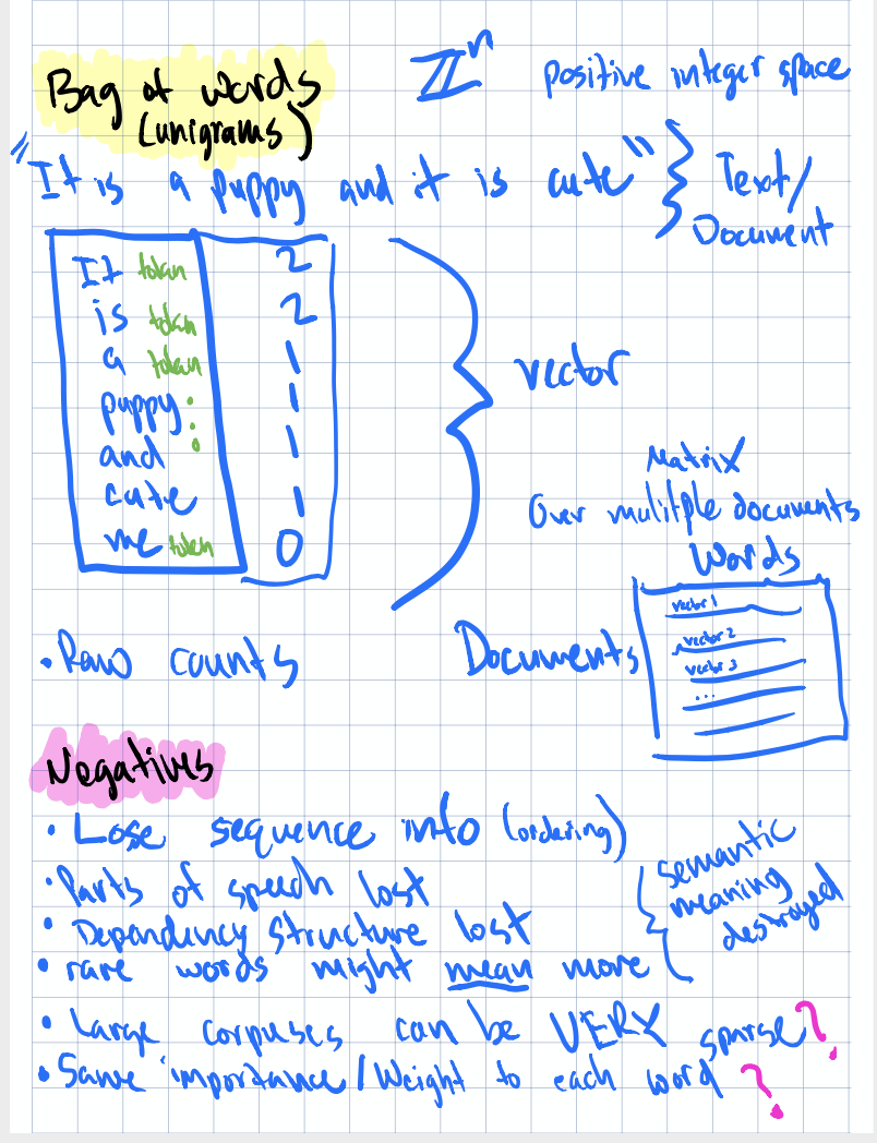
 BOW Example, Pros, & Cons
What excited me about this is featurization technique is how operationally straightforward it is. I’m pretty sure raw counts of each word in text documents could be handled natively in the warehouse for large corpuses. Imagine using a UDF that tokenizes and counts words across millions of user comments while tokenizing only for a specific set of negative/positive words; that’d be a pretty cheap an easy feature to identify comments worth flagging for review. Just think, a SQL-native approach could be a game changer for teams that don’t want to spin up a separate NLP pipeline just to get basic text features into their models.
Bag-of-n-Grams
The natural extension of BOW is to count not just individual words, but sequences of $n$ words (n-grams). Bigrams capture two-word phrases like “machine learning” or “not good” and that second example is exactly why n-grams can matter more than just BOW. Think about it, BOW treats “not” and “good” as independent signals; a bigram model understands “not good” as its own singular dimension.
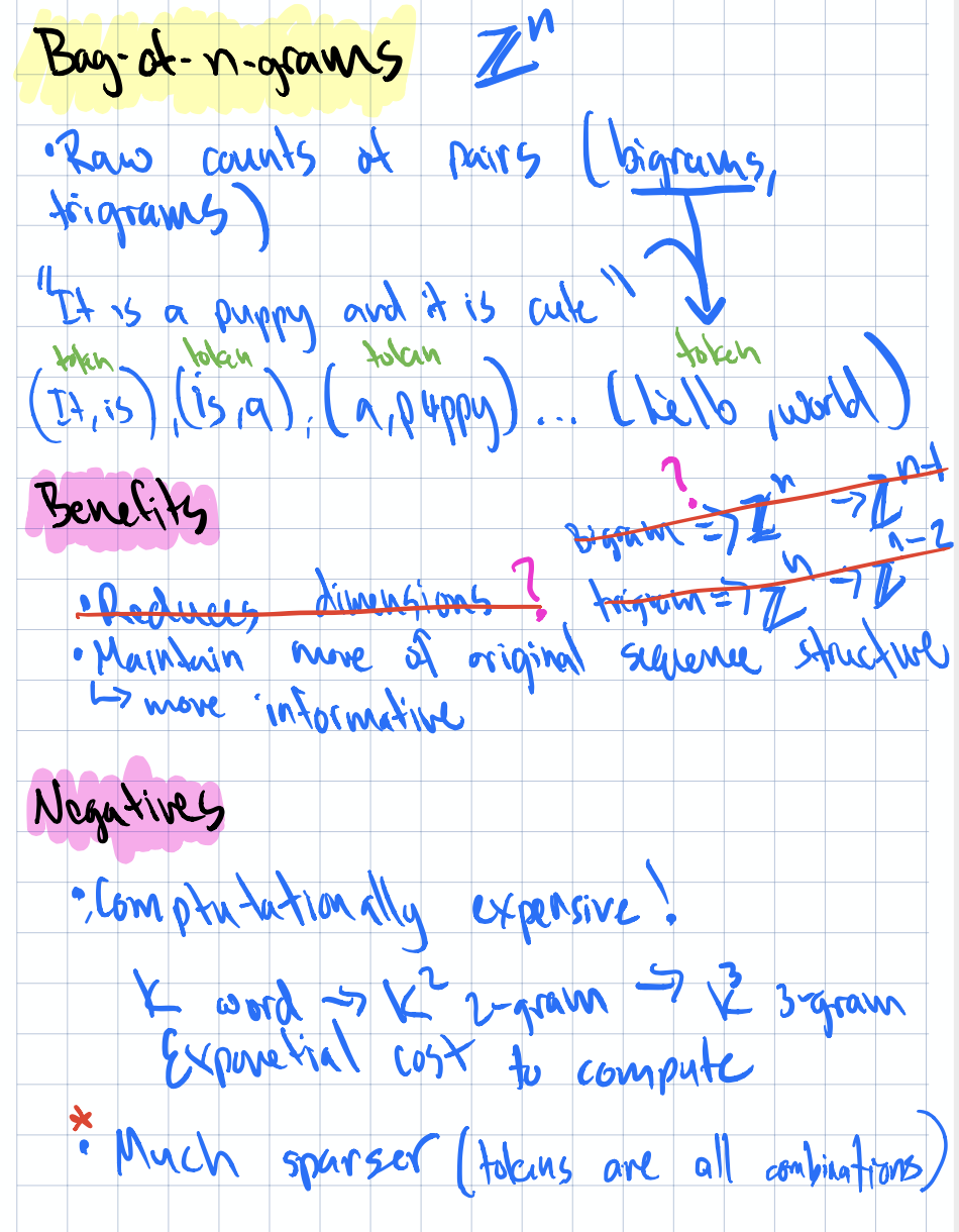 Diagram showing n-gram construction
Again, I found myself wondering: how easy would this be to implement in our data warehouse? The sliding window logic for generating n-grams from tokenized text isn’t complex, but doing it at warehouse scale with large compute and efficient storage is where it gets interesting. Perhaps some NLP pipelines could be really simplified if we’re aiming for blunt features… but again, we have to be careful here because with higher n-grams comes sparse matricies so dealing with that sparsity is going to be very important for downstream usecases.
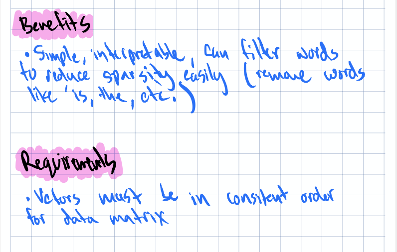
Filtering for Cleaner Features
As you can imagine, raw counts of words in bodies of text are noisy. Cleaning up that noise to get better signal from your text features can be done in a variety of ways. There’s the basic filter of course. For example, when we parse text, let’s just throw out words for anything that doesn’t have meaning downstream. If I’m trying to create features to cluster users by interest and I’m creating a “surfer” category from comments, or articles read, there are only so many words I’d consider a strong signal of this, all other words probably won’t help me there.
Stopwords
Stopwords like “the”, “is”, “and”, etc. tend to dominate word counts but carry little discriminative information. Removing them is a standard first step in boosting the level of useful information representated by your features.
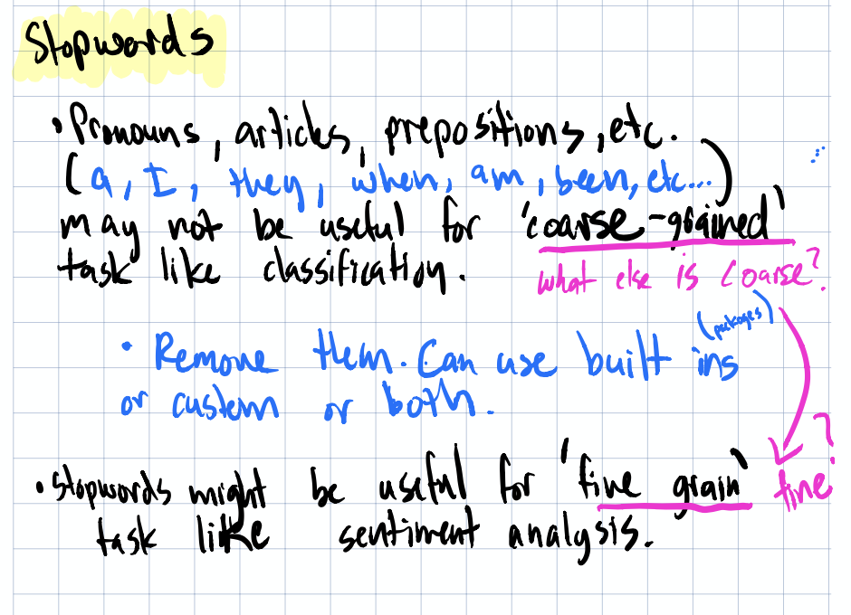
One thought I had here: how similar are the stopword lists across different domains? The stopwords for advertisements, journal articles, and user comments are probably pretty similar at the core, but each domain likely has its own “functional” words that carry no signal. It could be nice to have a centralized, open source, curated, “domain specific”, stopword list available as part of a text parsing toolchain; one less thing you’d have to think about if there were general consensus around it.
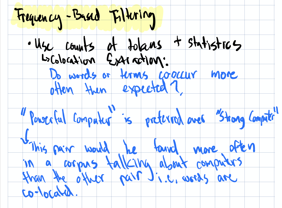
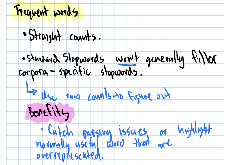
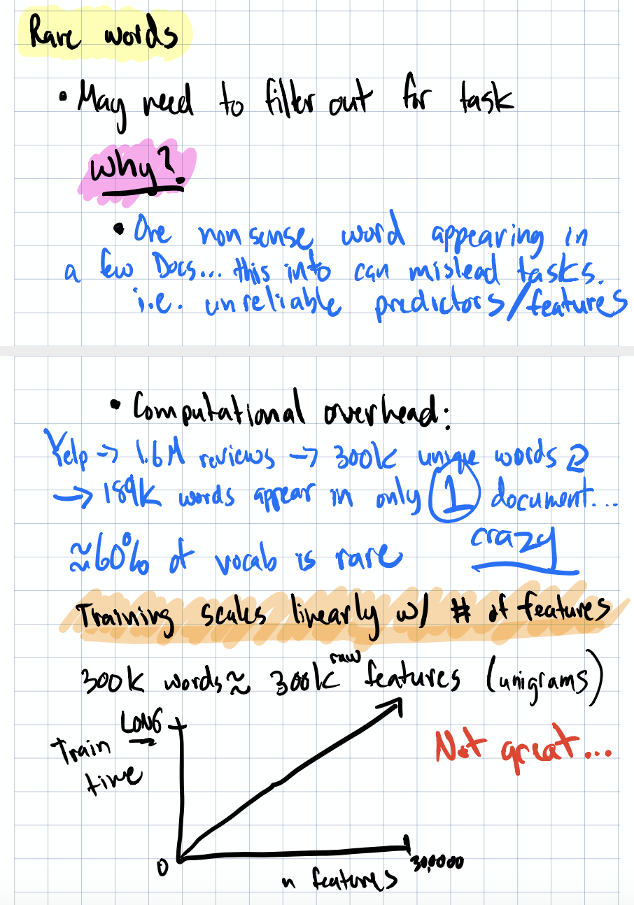
Frequency-Based Filtering
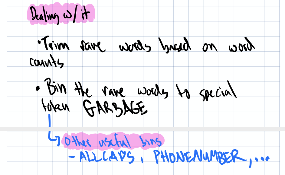
Beyond stopwords, you can filter by frequency more generally. Words that appear in nearly every document (too common) or in only one document (too rare) probably aren’t helping your model.
 Frequency filtering notes
One neat idea that came up: the GARBAGE token. After you’ve filtered out stopwords and rare/common words, if you still have a large count of tokens landing in a catch-all “garbage” bucket, that’s actually a useful diagnostic signal. It tells you to go back and look at the source documents — maybe there’s a pattern in the noise you’re missing, or your tokenization needs refinement.
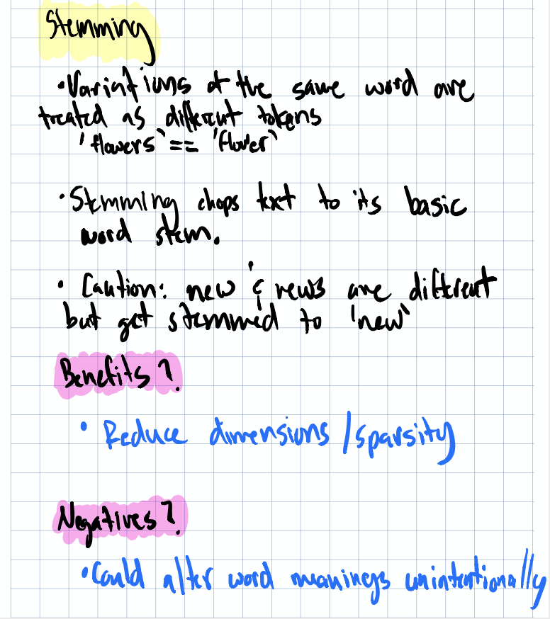
Stemming
Stemming reduces words to their root form — “running”, “runs”, “ran” all become “run”. This collapses your feature space and groups semantically similar words together.
 Stemming diagram
The tradeoff is that stemming can be aggressive and sometimes groups words that shouldn’t be grouped. But for reducing sparsity in your feature matrix, it’s a solid tool.
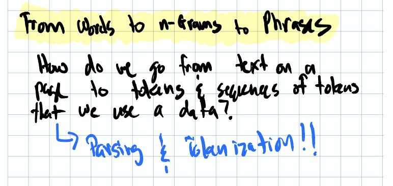
From Words to n-Grams to Phrases
There’s a natural progression from individual words → n-grams → meaningful phrases. The question is: at what point does the added complexity pay off?
 Words to phrases progression diagram
For many practical tasks (document classification, spam detection), BOW or bigrams are surprisingly competitive. But when you need to capture richer meaning,like understanding whether an ad headline is appealing to users, you’ll start wanting phrases and more structural features.
This connects directly to something I’ve seen in practice: teams experimenting with manipulating text headlines to get more user engagement. If you’re trying to understand what makes a headline click-worthy, simple word counts won’t cut it. You need to capture semantics as the specific phrasing matters, not just which words appear.
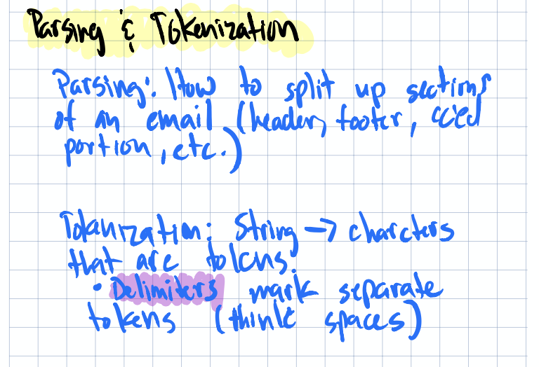
Parsing and Tokenization
Before we dive further on meaning phrases, you should familarize yourself with the differences between tokenization & parsing. Tokenziation is the process for breaking down text into words (or “tokens”) and parsing, is the process of analyzing word structure & grammer. When parsing text you can begin to leverage more complex structure such as parts of speech (POS), grammer, etc. This is where tools like SpaCy shine. Their tokenizers are highly extensible, letting you build in custom delimiters and rules for your specific domain.
 Parsing/tokenization diagram
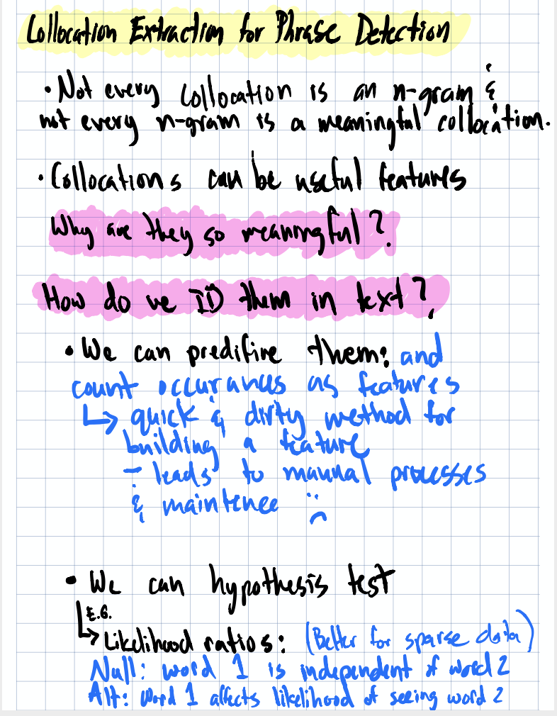
Collocation Extraction for Phrase Detection
Collocations are word pairs (or groups) that co-occur more often than chance would predict. “New York”, “machine learning”, “ice cream” — these are phrases where the individual words lose meaning if separated.
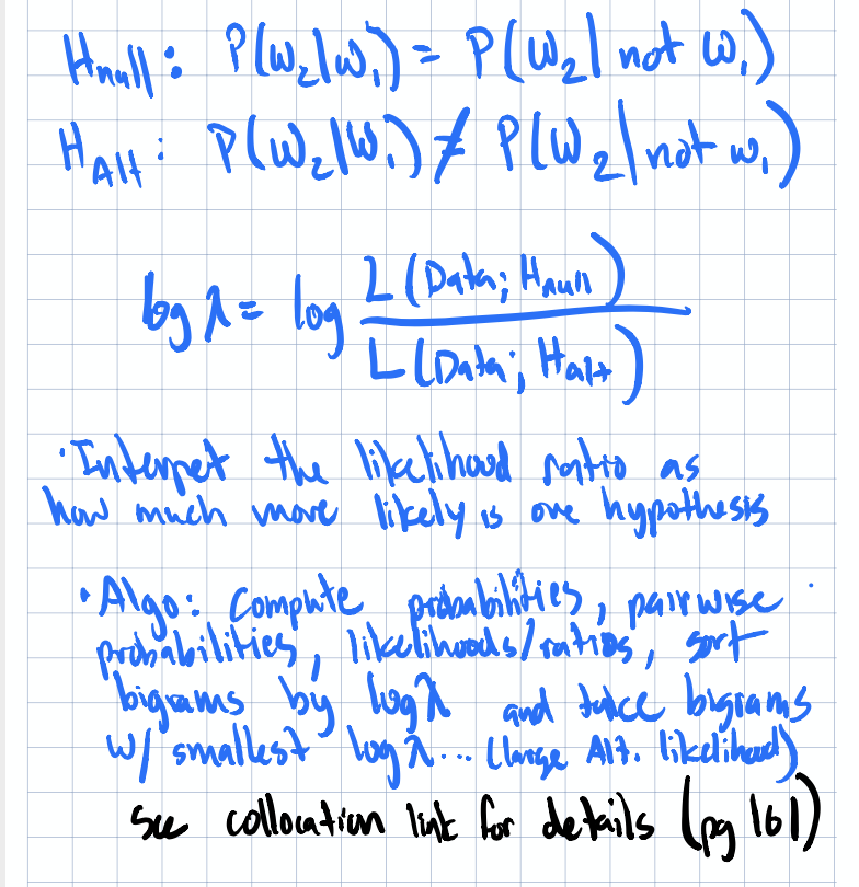
The statistical machinery behind collocation detection is fascinating. You’re essentially running hypothesis tests to determine whether two words appear together significantly more than their individual frequencies would suggest.
 Collocation Notes
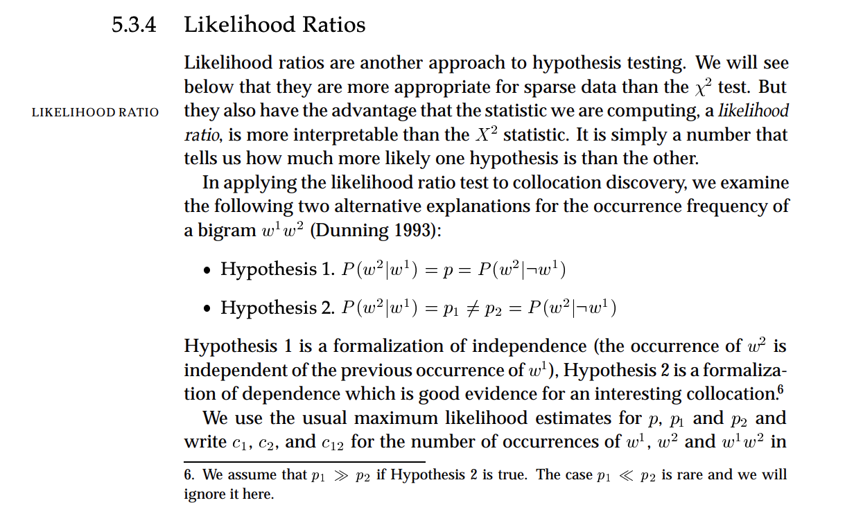
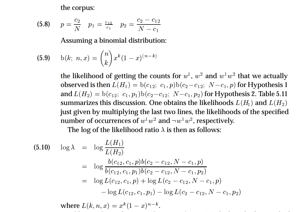
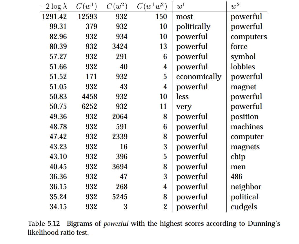 Collocation & Likelihood Ratios
I’ll be honest, I wanted more packages and tooling around collocation usage. The theory is well-established, but finding production-ready implementations that integrate cleanly into a feature pipeline took more digging than I expected.
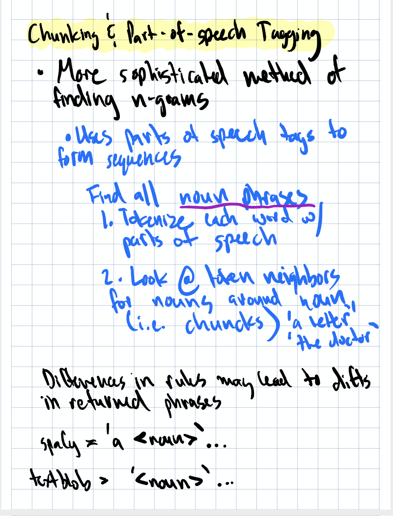
Chunking & Part-of-Speech Tagging
At the richest end of the spectrum, you can extract parts of speech (nouns, verbs, adjectives) and syntactic chunks from text. This preserves some of the hierarchical structure that count vectors throw away.
 POS tagging Notes
My take: POS tagging and entity extraction seem most valuable for specific, targeted tasks rather than general-purpose featurization. If you’re building a model to extract structured data from unstructured text (like pulling company names from job descriptions), POS tagging is invaluable. For broad classification tasks, the simpler methods usually win on the cost-benefit curve.
Fighting Sparsity: The Recurring Theme
If there’s one thread running through this entire chapter, it’s data sparsity. Text naturally produces extremely sparse feature matrices as most documents use only a tiny fraction of the total vocabulary in your corpus. Here are strategies for dealing with this that we’re covered:
- Filtering stopwords to remove low-signal dimensions
- Frequency-based filtering to prune rare and ubiquitous terms
- Stemming to collapse related words
- Binning with parts of speech - count all nouns, all adjectives, etc. as aggregate features
- Dimensionality reduction techniques (covered in a later chapter)
- Oversampling — create bigrams from your text, treat the set of all bigrams as a population, and bootstrap sample from it
Each of these has tradeoffs, and the right combination depends on your data and task.
Summary
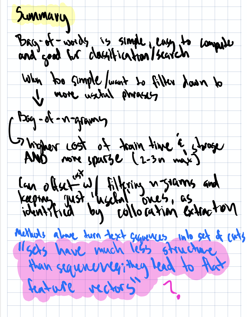
The progression in this chapter is clean: words → counts → filtered counts → n-grams → phrases → syntax. Each step adds richness but also complexity. For most practical applications, you’ll find that BOW or n-grams with good filtering gets you surprisingly far. The fancier techniques (collocations, POS tagging) are there when you need them, but they’re not always worth the overhead. Lastly, embeddings and sematics are the richest representation of all but they didn’t get that much coverage in this chapter.
The biggest insight for me was how much of text featurization is really about managing sparsity and that the simplest tools (stopword removal, frequency filtering, stemming) often have the highest ROI.
References
- Dependency Parsing Abbreviations (Stanford NLP)
- spaCy POS Tagging
- The Illustrated Word2Vec — excellent visual guide to embeddings
- Collocation Hypothesis Testing (Stanford NLP)
Next up in Part 3: we’ll start leveraging text for classification task.