The Normal Equation: Part 1 - Formulating the Cost Function
I’ve never found a blog post that truly made me understand how to derive the normal equation. I think a reason for this is a lot of authors have their own perspective on the problem, leading to a mental image I can’t quite grasp onto. But having grappled with linear algebra for a bit, I think I’m ready to try my hand at writing a series of posts that helps someone like my former self understand such an equation.
In this first post I’ll come up with an intuition for formulating the cost function we always see when talking about regression. I assume you know what a vector is and how to add/subtract them, what the span of a matrix/vector is, linear transformations, and norms. We won’t do any calculus until the next post so no need for that here.
The line of best fit
2 Dimensions
The idea behind the normal equation is it’s the analytical solution to a regression problem where you’re trying to find the line of best fit through your data, like the firgure below.
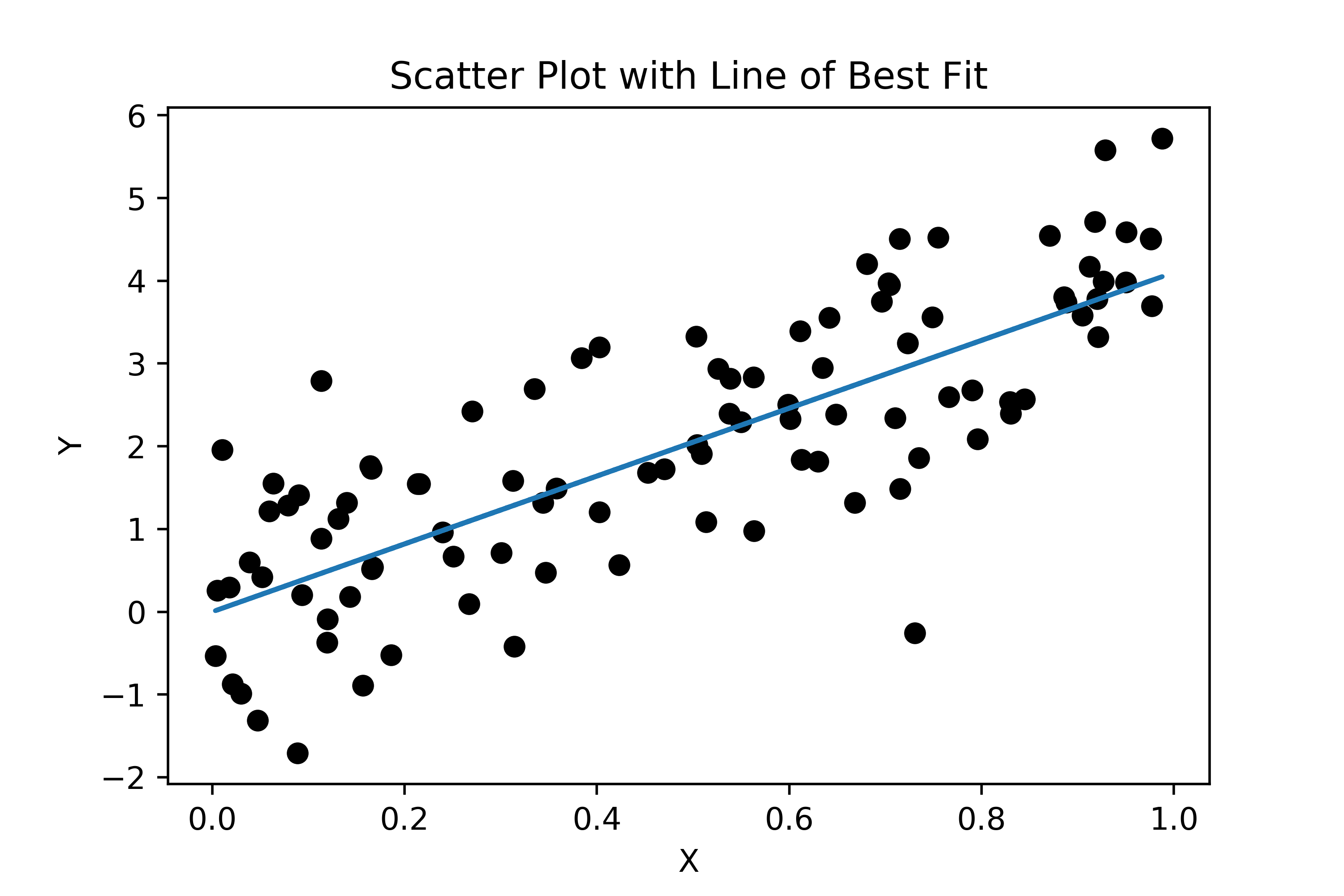
In two dimension we can express the line above with the equation: $$\color{black}\vec{y}=m\vec{x}+b$$
Where:
- $\color{black}\vec{y}$ is a column vector of observations
- $\color{black}\vec{x}$ is a column vector for a single covariate
- $\color{black}b$ is a scalar representing the intercept for the line (we’ll assume 0 here) and
- $\color{black}m$ is also a scalar representing the slope of the line
This is a great way to visualize the equation, however, once you start adding more covariates we need to stop thinking about the line of best fit and think more about the (hyper)plane of best fit.
N Dimensions
Below we depict an analagous figure to the line of best fit
but extended into 3 dimensions.
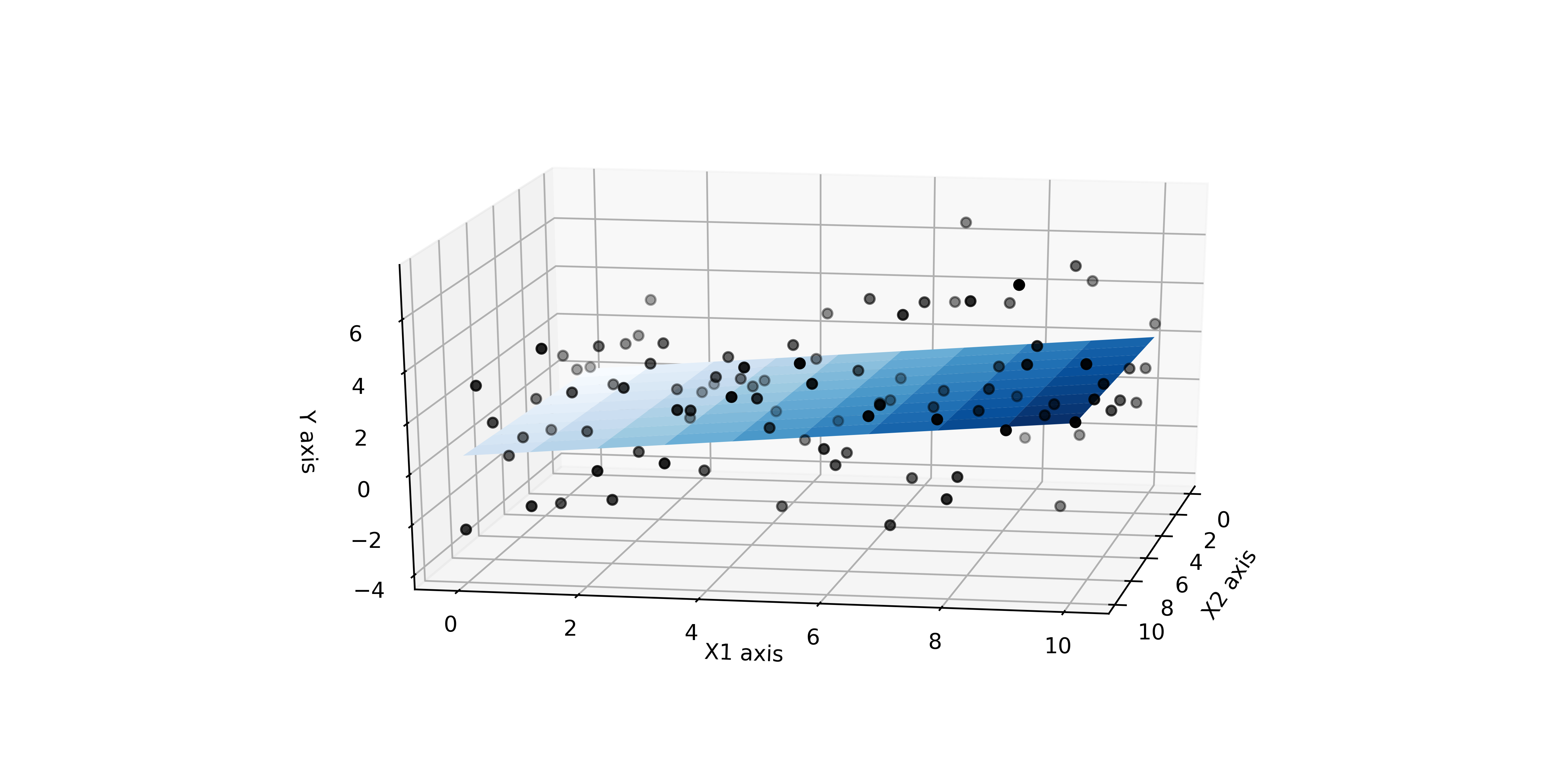
In order to represent the hyperplane that’s passing through this data we can simply change our 2D notation into 3D with matrices like so:
$$ \color{black} \vec{y} = A\vec{\theta} + b $$
Where:
- $\color{black}\vec{y}$ is your column vector of m observations
- $\color{black}A$ is m x n matrix of n covariate columns vectors
- $\color{black}\vec{\theta}$ is a n x 1 column vector of regression coefficients and
- $\color{black}b$ is scalar intercept.
To simplify further, we could could include the intercept ($\color{black}b$) within the coefficient vector $\color{black}\vec{\theta}$ and remove it from the above equation so $\color{black}\vec{\theta}$ will now look like this,
and the equation for our ‘plane’ of best fit simplifies to a matrix vector multiplication:
$$ \color{black}\vec{y}=A\vec{\theta}\tag{1} $$
Defining the Cost Function
The way I like to look at equation $\color{black}(1)$ is to think of the matrix $\color{black}A$ as a linear map, transforming our column vector $\color{black}\vec{\theta}$ to match the same vector as $\color{black}\vec{y}$ (i.e. span the same space). But in order to transform $\color{black}\vec{\theta}$ into $\color{black}\vec{y}$ we need to first find the right combination of parameters to map into the space of $\color{black}A$ (i.e. find the optimal $\color{black}\vec{\theta}$’s). And the way we can find this combination of parameters is with our good friends calculus and geometry.
But before we start taking derivates of a function to find the optimal $\color{black}\vec{\theta}$, we need to define the function we’re going to optimize (i.e. the cost function $\color{black}J(\vec{\theta})$). We can create a cost function for equation $\color{black}\color{black}(1)\space\space\vec{y}=A\vec{\theta}$ by thinking about minimizing the difference vector between $\color{black}\vec{A\theta}$ and $\color{black}\vec{y}$; think of the resulting vector you get when doing vector subtraction because $\color{black}\vec{A\theta}$ is a vector as defined by it’s dimensions just as much as $\color{black}\vec{y}$ is a vector.
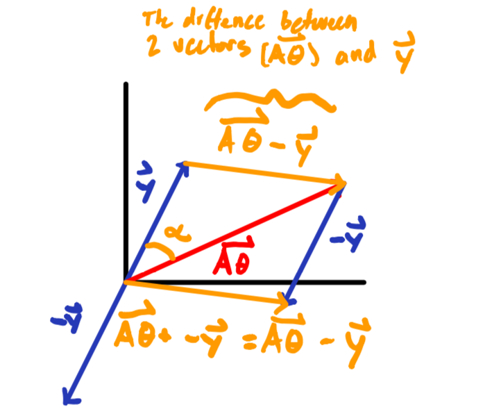
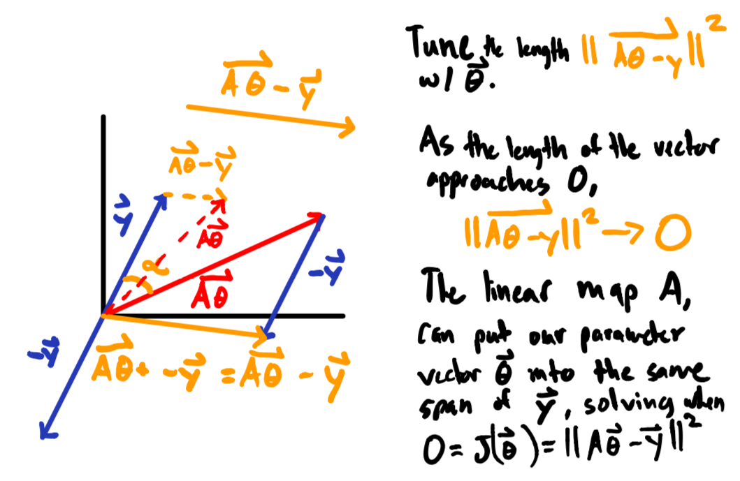
And now think of representing the difference vector in orange above ($\color{black}\vec{A\theta}-\vec{y}$) as one big vector itself $\color{black}\vec{A\theta-y}$ (see below), and we can really start to play with our perspective on the cost function $\color{black}J(\vec{\theta})$ to be.
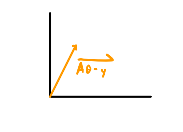
From a geometric viewpoint we want to know how long our big expression vector in orange above is i.e. the length of $\color{black}\vec{A\theta-y}$. The nifty thing about measuring a vector is it’s the same thing as taking the dot product with itself.
$$ \color{black}(\vec{A\theta-y})\cdot(\color{black}\vec{A\theta-y}) $$ Because $$ \color{black}(\vec{A\theta-y})\cdot(\color{black}\vec{A\theta-y}) = \cos(\alpha)\space||\vec{(A\theta-y)}||\space|| \vec{(A\theta-y)}|| $$ And when you’re dotting a vector with itself, the angle ($\color{black}\alpha$) between a vector and itself is 0 so the dot product expression $$ \color{black}(\vec{A\theta-y})\cdot(\color{black}\vec{A\theta-y}) = \cos(0)\space||\vec{(A\theta-y)}||\space|| \vec{(A\theta-y)}|| $$ simplies to this, $$ \color{black}(\vec{A\theta-y})\cdot(\color{black}\vec{A\theta-y}) = \space||\vec{(A\theta-y)}||\space|| \vec{(A\theta-y)}|| $$ because the $\color{black}cos(0)=1$ and this turns out to be the L2 norm of $\color{black}(\vec{A\theta - y})$ (i.e. the norm squared). $$ \color{black}(\vec{A\theta-y})\cdot(\color{black}\vec{A\theta-y}) = \space||\vec{(A\theta-y)}||^2\tag{2} $$
So it turns out the we can measure the length of the vector represented by our expression, $\color{black}(\vec{A\theta - y})$, through the $\color{black}L2$ norm and that allows us to define our cost function $\color{black}J(\vec{\theta})$. $$ \color{black}J(\vec{\theta})=||A\vec{\theta}-\vec{y}||^2\tag{3} $$
And when we want to find a set of parameters $\color{black}\vec{\theta}$ that minimizes our ‘difference’ vector in orange (above), we have an optimization problem (which is where calculus comes in).
Visual Intuition of the Cost Function
Now that we know how to define our cost function as a optimization problem that minimizes the length of vector ($\color{black}\vec{A\theta - y}$) representing the difference between, $\color{black}\vec{y}$ and $\color{black}\vec{A\theta}$ we can come up with a visual to help intuit the process.
The Cost Function Rearranged
While the formulation of our cost function in equation $\color{black}(3)$ is intuitively nice, it doesn’t help us actually solve the optimization problem involved with finding the parameter vector $\color{black}\vec{\theta}$.
To make our cost function $\color{black}J(\vec{\theta})$ more amenable to solving with calculus and derivatives, lets get rid of the squared component. Remember, according to equation $\color{black}(2)$, $\space\space\color{black} (\vec{A\theta-y})\cdot(\vec{A\theta-y}) = \space||\vec{(A\theta-y)}||^2$, the $\color{black}L2$ norm is the equivalent to the dot product and you can rewrite the dot product in terms of multiplication between a row and column vector, $$ \color{black}J(\vec{\theta})= \space||\vec{(A\theta-y)}||^2= (\vec{A\theta-y})\cdot(\vec{A\theta-y})= \color{black}(\vec{A\theta - y})^T (\color{black}\vec{A\theta - y}) $$
And because we used a big vector notation above, we can shift our perspective down to the indiviual vectors and rewrite the cost function as this: $$ \color{black}J(\vec{\theta})=(A\vec{\theta} - \vec{y})^T(A\vec{\theta} - \vec{y}) $$
Where we can now distribute the transpose which you can think of as an operator that just rotates vectors, and rearrange terms to reflect rotated vectors, $$ \color{black} = ((A\vec{\theta})^T - (\vec{y})^T)(A\vec{\theta} - \vec{y}) $$ $$ \color{black} = (\vec{\theta}^TA^T - \vec{y}^T)(A\vec{\theta} - \vec{y}) $$
Then do the multiplcation (making sure the terms stay in the proper
order)
$$
\color{black} = \vec{\theta}^TA^TA\vec{\theta} -
\vec{y}^TA\vec{\theta} -
\vec{\theta}^TA^T\vec{y} -
\vec{y}^T\vec{y}
$$
And with one more rearragnement, remebering that $\color{black}(A\vec{\theta})^T = \vec{\theta}^TA^T$, we can take the transpose of this whole term $\color{black}(\vec{y}^TA\vec{\theta})^T$ and we’ll get this, $$ \color{black} = \vec{\theta}^TA^TA\vec{\theta} - \vec{\theta}^TA^T\vec{y} - \vec{\theta}^TA^T\vec{y} - \vec{y}^T\vec{y} $$ Which simplifies our cost function to a form where we can now solve the optimization problem with derivates: $$ \color{black}J(\vec{\theta}) = \vec{\theta}^TA^TA\vec{\theta} - 2\vec{\theta}^TA^T\vec{y} - \vec{y}^T\vec{y}\tag{4} $$
And there you have it, the cost function visualized, defined, and ready for optimization. In the next post we’ll cover how to solve this system of equations i.e. find the analytical solution to $\color{black}\nabla J(\vec{\theta})=0$
Fin
Thanks for reading.There were a number of resources involved in helping me come up with this perspective and here’s a few for you to checkout yourself: